Predicting diabetic patient readmission with machine learning

Figure 1: Photo by Artem Podrez from Pexels
Hospitals and clinics see early hospital readmission of diabetic patients as a worldwide, high-priority health care quality measure and target for cost reduction. “Early readmission” here is understood by any another hospital admission of the same patient within 30 days of discharge. The choice of a 30-day window as a measure of readmission is because such length of time is likely attributable to the quality of care during the index hospitalization, thus representing a preventable outcome. (Graham et al., 2018)
The costs of early readmission are huge. Given that one in five Medicare beneficiaries is readmitted within 30 days in the U.S., more than $26 billion are spent per year, with diabetes being one of the most significant risk factors that contribute to this scenario. (Soh et al., 2020)
In 2012, The Patient Protection and Affordable Care Act in the United States established that Centers for Medicare and Medicaid Services (CMS) would impose financial penalties on hospitals for excessive readmissions within 30 days of hospital discharge. Thus, to encourage improvement in the quality of care and reduce unnecessary health expenses, policymakers, reimbursement strategists, and the United States government have made reducing 30-day hospital readmissions a national priority.
Therefore, a complete understanding of the underlying causes of readmission is needed to reduce its rate, so any insights we can gather from this scenario could positively impact health policies.
Assumptions
Why would a patient be early readmitted in the first place? Here are a few hypotheses:
- Patients are not adequately diagnosed as diabetic on the first admission;
- Ineffectiveness of treatment during past hospitalizations, namely
- insufficient number of exams;
- insufficient medical intervention (medication change or procedures);
- Poor patient health.
One study showed that patients often felt that their readmissions were preventable and linked them to issues with “discharge timing, follow-up, home health, and skilled services” (Smeraglio et al., 2019)
Patient characteristics such as gender, age, race, and comorbidities, may affect the outcomes (Soh et al. 2020), so they could be used to model early patient readmission. Furthermore, a well-known index adopted by health practitioners called LACE takes into account four other variables:
- the length of stay;
- whether the patient was admitted through the emergency department or came voluntarily;
- whether or not the patient has more than one disease or disorder;
- and the number of emergency department visits in the previous six months before admission.
All these are a good baseline to start with. Nevertheless, other variables could also be assessed, such as:
- type of prescribed medication;
- whether hospitals successfully discharged patients to their home;
- most frequent comorbidities among diabetic and non-diabetic patients;
- number of medical interventions during the inpatient setting.
Objective
In this work, I will try to answer the following questions:
- Are readmitted diabetic patients correctly diagnosed in their first admission?
- Given that HbA1c values are vital for planning the diabetic patient’s medication (according to the literature), how often doctors ask for HbA1c tests in the inpatient setting?
- Are readmitted diabetic patients receiving an appropriate medical intervention, like change in their medication or medical procedures if need be?
- Which variables are the strongest readmission predictors?
And finally, would it be possible to create a predictive model for early readmission?
Such a model could help plan interventions for high-risk patients and reduce emotional and financial costs for both patients and hospitals, respectively. Again, the target variable will be unplanned readmissions that happen within 30 days of discharge from the initial admission since this is the field standard.
The proposed predictive model should be interpretable, which is to say that health practitioners can understand why the model comes to a particular prediction, and whether the variables had a positive or negative effect on the outcome, and to which extent. That being said, the most appropriate model for the job would be either logistic regression, which returns calibrated probability as its results and gives a detailed view on how each feature affects prediction, or a random forest classifier. Although the latter is a more robust model and returns to which extent each variable affected the model’s prediction, it is considerably slower to converge.
Early hospital readmission seems to incur higher costs to a hospital when compared to a patient’s longer length of stay or enhanced preventive measures. Therefore, we should aim to minimize false negatives, and the most appropriate metric, in this case, would be recall. But a high recall metric is not telling enough. Theoretically, we could strive toward a near-perfect recall value at the expense of poor precision (more false positives). Unfortunately, field knowledge is required to assess a tolerable false positives rate, which can vary from hospital to hospital. Since we lack this information, this work will use the area under the ROC curve as the primary metric. Optimizing for ROC will guarantee that both true positives rate and false positives rate will be maximized, and then the decision of an appropriate cut-off value will be up to the health practitioner.
For more information, please check out my Github repository containing the Jupyter notebook for technical details.
Data characteristics
The data set used for this task is the
Diabetes
130-US hospitals for years 1999–2008 Data Set, containing anonymized
medical data collected during 100k encounters across several hospitals
in the United States, made available by Strack et al. (2014). It
comprises two files, diabetic_data.csv and IDs_mapping.csv. The
former contains the medical data itself, and the latter contains a
legend for some of the numerical categories (like admission type and
discharge disposition).
Here’s a description of each feature in the data set:
- Encounter ID — Unique identifier of an encounter
- Patient number — Unique identifier of a patient
- Race Values — Values: Caucasian, Asian, African American, Hispanic, and other
- Gender Values — Values: male, female, and unknown/invalid
- Age Grouped in 10-year intervals — 0, 10), 10, 20), …, 90, 100)
- Weight — Weight in pounds
- Admission type — Integer identifier corresponding to 9 distinct values, for example, emergency, urgent, elective, newborn, and not available
- Discharge disposition — Integer identifier corresponding to 29 distinct values, for example, discharged to home, expired, and not available
- Admission source — Integer identifier corresponding to 21 distinct values, for example, physician referral, emergency room, and transfer from a hospital
- Time in hospital — Integer number of days between admission and discharge
- Payer code — Integer identifier corresponding to 23 distinct values, for example, Blue Cross/Blue Shield, Medicare, and self-pay Medical
- Medical specialty — Integer identifier of a specialty of the admitting physician, corresponding to 84 distinct values, for example, cardiology, internal medicine, family/general practice, and surgeon
- Number of lab procedures — Number of lab tests performed during the encounter
- Number of procedures — Numeric Number of procedures (other than lab tests) performed during the encounter
- Number of medications — Number of distinct generic names administered during the encounter
- Number of outpatient visits — Number of outpatient visits of the patient in the year preceding the encounter
- Number of emergency visits — Number of emergency visits of the patient in the year preceding the encounter
- Number of inpatient visits — Number of inpatient visits of the patient in the year preceding the encounter
- *Diagnosis 1 — The primary diagnosis (coded as first three digits of ICD9); 848 distinct values
- Diagnosis 2 — Secondary diagnosis (coded as first three digits of ICD9); 923 distinct values
- Diagnosis 3 — Additional secondary diagnosis (coded as first three digits of ICD9); 954 distinct values
- Number of diagnoses — Number of diagnoses entered to the system 0%
- Glucose serum test result — Indicates the range of the result or if the test was not taken. Values — “>200,” “>300,” “normal,” and “none” if not measured
- A1c test result — Indicates the range of the result or if the test was not taken. Values: “>8” if the result was greater than 8%, “>7” if the result was greater than 7% but less than 8%, “normal” if the result was less than 7%, and “none” if not measured.
- Change of medications — Indicates if there was a change in diabetic medications (either dosage or generic name). Values: “change” and “no change”
- Diabetes medications — Indicates if there was any diabetic medication prescribed. Values: “yes” and “no”
- 24 features for medications — columns named after diabetes-related medication indicating whether the drug was prescribed or there was a change in dosage. Values: “up” if the dosage was increased during the encounter, “down” if the dosage was decreased, “steady” if the dosage did not change, and “no” if the drug was not prescribed
- Readmitted — Days to inpatient readmission. Values: “❤0” if the patient was readmitted in less than 30 days, “>30” if the patient was readmitted in more than 30 days, and “No” for no record of readmission
Missing values are represented by question marks in the tables, and
except for weight, payer_code, and medical_specialty (which were
dropped from the data for this study), there are very few missing
values.
The data set is moderately unbalanced, with the positive class
(readmitted = "<30") comprising 11% of the data set. By evaluating the
number of patients to whom diabetes medication was prescribred during
the inpatient settings, we can spot several low-variance features with
the naked eye (like metformin-rosiglitazone and metformin-ploglitazone
at the bottom of the list).
Diagnosis frequency among the readmitted and non-readmitted patients
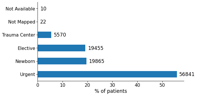
Figure 2: Common primary diagnosis codes among non-readmitted and readmitted patients. Blue bars indicate the most significant diagnosis that is present in one group and not in the other.
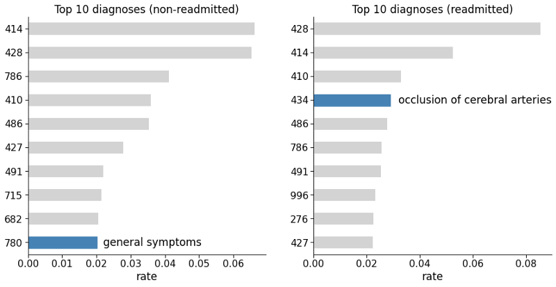
We can see that “general symptoms” (code 780) is among the top ten diagnoses for non-readmitted patients, but not for the readmitted ones. While “occlusion of cerebral arteries” (code 434) is among the top ten diagnoses for readmitted patients but not for the non-readmitted ones. Therefore these variables seem to contain great predictive information, and thus will feed the models at the end of the study.
IDs Mapping
Taking a look at IDs_mapping.csv, the file isn’t in standard CSV
format. It’s actually a text file mapping numerical categories to
strings in regard to the kind of hospital admission. With this file I
could replace each ID with the appropriate names in the original
dataframe.
Figure 3: Occurrences of different types of admission in the data set.
More data set characteristics
- The data set covers a 10-year span (1999–2008).
- Hospital admissions in the data set are supposed to be diabetic-related only, but some entries don’t have a diabetes-specific ICD-9 code (250.xx). I suppose that, maybe, such diagnosis was made during readmission, which is the reason for it not to show up sometimes.
- Lab tests were performed during admission.
- Medications were administered during admission.
- Data set contains multiple readmissions of the same people.
- Lots of low-variance variables in this data set (e.g.
examideandcitogliptonhave only 1 unique value), which won’t add to the model’s predictive power. diag_1todiag_3columns have too many ICD-9-CM codes and will have to be grouped.
Missing values:
weightvariable is nearly useless, with about 97% of missing values.payercodecould be an useful variable, but has a concerning number of missing values (around 40%)medical_specialtyhas half of its values missing.
Target variable: 30-day remission, i.e. unplanned or unexpected readmission to the same hospital within 30 days of being discharged.
Data preparation
Remove duplicates
A few rows in the data set refer to the same patient number
(patient_nbr). Most machine learning models require the observations
to be independent of each other. More specifically, the assumption is
that observations should not come from repeated measurements. To ensure
our model’s robustness, duplicated entries for the same patient were
deleted (while keeping the first appearance only).
Drop unneeded features
encounter_id,patient_nbr, andpayer_code: irrelevant to patient outcomeweight,medical_specialty: too many missing values.admission_source_id: redundant variable (admission_type_idalready contains information about the admission)- all medications (including the most common: metformin, glimepiride,
glipizide, glyburide, pioglitazone, rosiglitazone, and insulin): they
either correlated strongly with
diabetesMed, which indicates if there’s any diabetic medication prescribed, or not used at all.
Transform individual features
Age: The age group feature in this data set is categorical, but can be turned into an ordinal variable. That way we avoid creating too many new features after the one-hot encoding process.
age_map = {'[0-10)': 0,
           '[10-20)': 1,
           '[20-30)': 2,
           '[30-40)': 3,
           '[40-50)': 4,
           '[50-60)': 5,
           '[60-70)': 6,
           '[70-80)': 7,
           '[80-90)': 8,
           '[90-100)': 9}
Gender: Genders were converted to either 0 if male or 1 if female.
Admission type ID: There are 9 distinct values in this column. I grouped this feature by whether patients were admitted in an emergency or not. Thus, “Emergency” (which includes the “Urgent” label) became 1 and everything else will be 0.
Discharge disposition ID: This feature has 29 distinct features, which would negatively impact the model’s performance if we create dummy values for all of them. Therefore, I restricted these values to either “discharged to home” or other.
Diagnosis: The diagnosis features are represented by ICD-9 codes. The idea here is to condensate the hundreds of codes into just a few major groups, based on field knowledge (Strack et al., 2014). I also made sure to include the diagnoses that were among the top 10 for readmitted patients but not for non-readmitted, and vice-versa.
Glucose serum test result (max_glu_serum) and A1c test: This variable indicates the range of the test results, or whether the tests were taken at all. It could be be converted into an ordinal variable and spare the creation of unnecessary dummy features.
Also, according to the literature (Strack et al., 2014), adjusting the
patient’s medication according to HbA1C levels can diminish early
readmission rates. Therefore, this new variable is going to be
incorporated into the model, and will be 0 if A1Cresult is “none” or 1
otherwise.
Change of medication and diabetes medications: the categorical object type was simply converted to numerical.
Readmitted (target variable): value is 1 if readmitted earlier than 30 days, 0 otherwise.
Dummy variables creation
All categorical variables were converted into dummy variables (one-hot encoding).
Merging diag_n variables
The diag features represent what the physician thought would be the
causes of the patient admission. As a rule, the primary (principal)
cause of admission should be the diag_1 variable. diag_2 and
diag_3 variables are left for secondary causes. To avoid passing too
many dummy variables to the model, I merged the three features into a
weighted sum. Example: if a patient has diag_1_Circulatory = 1,
diag_2_Circulatory = 1, and diag_3_Circulatory = 0, the weighted sum
is going to be diag_Circulatory = 1x3 + 1x2 + 0x1 = 5.
Analysis of correlated variables
A final check for correlated variables was performed to see if any one variable could cause a large amount of problem to the model’s prediction. Highly-correlated variables (more than 0.9) may result in unstable models. This is especially true for logistic regression models.
A1C_tested            A1Cresult               0.917508
A1Cresult             A1C_tested              0.917508
max_glu_serum         max_glu_serum_tested    0.902445
max_glu_serum_tested  max_glu_serum           0.902445
race_Caucasian        race_AfricanAmerican    0.807590
race_AfricanAmerican  race_Caucasian          0.807590
change                diabetesMed             0.506697
diabetesMed           change                  0.506697
As expected, A1Cresult is strongly correlated with the engineered
feature A1Ctested. The same is valid for max_glu_serum_tested and
max_glu_serum.
After a few tests, I concluded that these values were not sufficient to affect the models’ performance (and in fact, even helped them).
Model implementation
Contrary to the random forest classifier, logistic regression models are particularly sensible to convergence problems. In this study, the LR model comprises several pre-processing steps:
- Standardizing the training set to guarantee a faster convergence. In
this study, I had to resort to the saga algorithm, which is the only
one that works with both L1 and L2 regularization in the Scikit-learn
library. However, saga fast convergence is only guaranteed on features
with approximately the same scale.
- Dropping variables that have null variance. Since they do not contain
any relevant information, they won’t add to the final result.
- Selection of the most relevant features based on ANOVA test between
each feature and the target variable. ANOVA was the test of choice because of speed, and also because the chi2 test requires values to be positive, which would not work after the StandardScaler process them. There are workarounds (like using Sklearn’s MaxAbsScaler function if chi2 is absolutely necessary).
- To ensure convergence, the classifier’s parameter
max_iter(maximum
number of iterations) was changed from 100 to 1000.
These steps were encapsulated with help from Scikit-learn’s Pipeline method, which guarantees that the model will always predict outputs using the same parameters from the training stage.
The Random Forest classifier is a bit more robust when it comes to convergence, so that scaling the data isn’t a pre-requisite in most cases.
Given class imbalance in the data set, both logistic regression and
random forest classifier models had the parameter class_weight set to
“balanced”. But since I configured the grid search to optimize for ROC
AUC, which is a class imbalance tolerant metric, this option has barely
budged the final results.
Refinement
Hyperparameters optimization is a key step for every machine learning project since not all data is born equal, and Scikit-learn’s defaults are rarely the best choice when it comes to performance. This is specially true with the random forest classifier, which doesn’t come with a hard limit for how deep trees can grow, resulting in overfitting.
A grid search was performed for both classifiers with the following search space:
# Perform Logistic Regression grid search.
lr_params = {
        "select__k": range(2, X.shape[1]),
        'clf__penalty':["none", "l2", "l1"],
        'clf__C': np.logspace(-3,3,7)
    }
# Perform Random Forest Classifier grid search.
rf_params = {
    "criterion": ["gini", "entropy"],
    "max_depth": [8, 13, 21, 34, 55],
    "min_samples_split": [55, 89, 144, 233],
    "min_samples_leaf": [3, 5, 8, 13, 21, 34],
    "max_features": ["sqrt", "log2", None],
    "oob_score": [True, False],
}
The grid search was relatively fast for LR, but took hours to complete for the RF. The reason is obvious: the model’s execution time is directly linked to the number of estimators instantiated by the random forest classifier. The more trees to be trained, the longer the time it will take to complete.
Evaluation
These are the metrics of the Logistic Regression model when tested against the testing set:
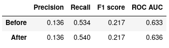
Figure 4: Logistic Regression, before and after optimization
And these are the metrics of the Random Forest model when tested against the testing set:
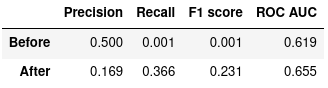
Figure 5: Random Forest Classifier, before and after optimization
The ROC curves below compare how each model performs with several different decision function thresholds.
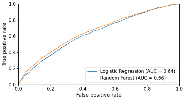
Figure 6: ROC curve of both Logistic Regression and Random Forest models.
Validation
To evaluate whether the optimized models are robust enough, I performed a 10-fold cross-validation. The table below shows how each model performed during CV with regard to ROC AUC values.
Logistic regression cross-validation
==========================================
Fold 0: 0.627
Fold 1: 0.627
Fold 2: 0.619
Fold 3: 0.627
Fold 4: 0.640
Fold 5: 0.632
Fold 6: 0.615
Fold 7: 0.643
Fold 8: 0.637
Fold 9: 0.629
------------------------
Mean ROC score: 0.630
Std. deviation: 0.008
Random forest classifier cross-validation
==========================================
Fold 0: 0.657
Fold 1: 0.633
Fold 2: 0.621
Fold 3: 0.651
Fold 4: 0.645
Fold 5: 0.645
Fold 6: 0.624
Fold 7: 0.654
Fold 8: 0.664
Fold 9: 0.649
------------------------
Mean ROC score: 0.644
Std. deviation: 0.01
The relative standard deviation of both models is less than 2%, which indicates both models are stable and don’t fluctuate much with small perturbations in the training data.
Discussion
The Random Forest classifier performed slightly better than the Logistic Regression in terms of ROC AUC, so we are going to use the latter’s coefficients (i.e. feature importances) as a basis for our analysis.
This is how each feature affected the machine learning model’s prediction:
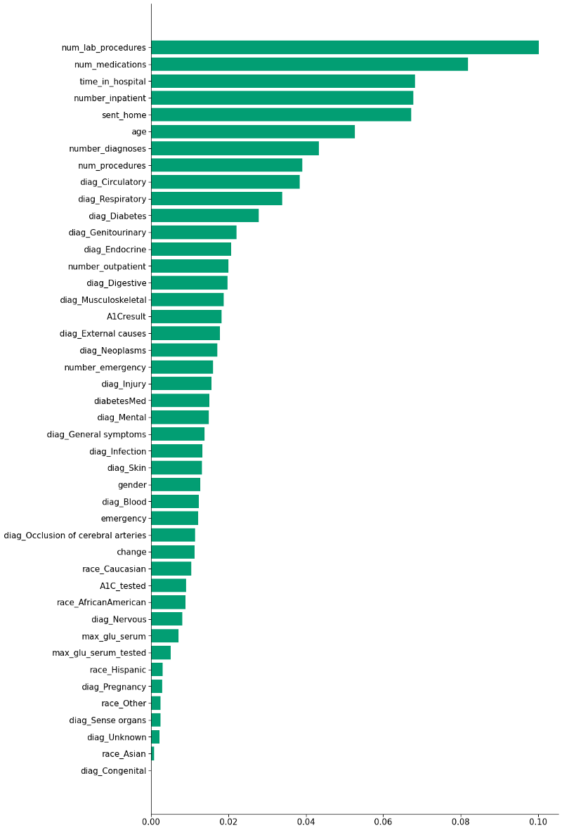
In an ensemble model like the Random Forest, every feature count as a vote in the final prediction, even if they are highly correlated or unimportant (although they may have a smaller weight in the decision). I’m going to focus on the 10 most important features according to the model:
time_in_hospital=*,* =num_lab_procedures=*,* =num_medications=*,* =number_diagnoses and num_procedures
These five variables are highly correlated, and it makes sense — the longer you stay in hospital, the more medications, lab procedures, diagnoses and general procedures you’re likely to be subjected to.
medications, diagnoses, and general procedures. 
Moreover, how does staying longer affect readmission? It seems that more extended hospital stays do not imply fewer readmissions. Quite the opposite: the longer the stay, the higher the likelihood of admission (see figure below).
It is impossible to tell if a prolonged stay worsens the patient’s health and increases their chance of readmission because correlation does not imply causation. Most likely, the longer stay is precisely a sign that the patient’s health is fragile, hence the higher probability of readmission within 30 days.
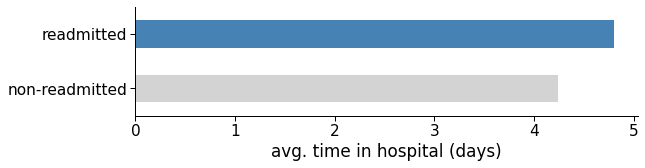
Figure 8: Average number of days in hospital for readmitted and non-readmitted patients.
number_inpatient
The number of inpatient visits in the year preceding the encounter. The model suggests that the more often patients have been admitted in the previous year, the higher the likelihood they will be readmitted in the future. Let us call this a darker version of the Lindy Effect: “if you were to a hospital last year, you would probably visit it next year too.”
That could be an indirect indicator of the patient’s health, which may correlate with the number of hospital visits.
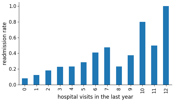
Figure 9: Readmission rate in function of number of hospital visits in the last year.
age
As expected, older patients are more prone to unexpected complications and, consequently, early readmissions. They also take longer to recover, as observed in the graph below. In that case, it is recommended that hospitals be more incisive with older patients regarding preemptive measures.
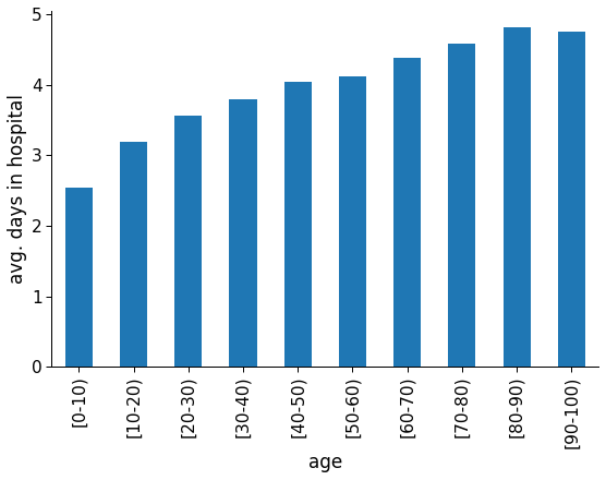
Figure 10: Average hospital stay length for each age group.
sent_home
The rationale behind this engineered feature was that going home instead of another short term hospital, skilled nursing facility or inpatient care institution (either due to discharge or continued treatment) could positively impact the patient’s recovery, so much so that they would be at lesser risk of readmission.
However, non-readmission does not necessarily mean recovery. There are other reasons for a patient not showing up, like giving up on electively going to the hospital again, being transferred to a hospice, or death.
Either way, this engineered feature was one of the most informative features according to the model and could be used at least partially to account for future readmissions. According to the data, around 60% of the readmitted patients had been sent home, versus more than 75% of the non-readmitted.
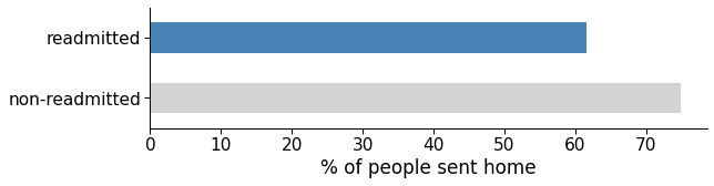
Figure 11: Average rate of people sent home in the readmitted and non-readmitted group.
Further questions
Now that we have treated the data set and trained a model, we can start answering other critical questions of this work.
Were readmitted diabetic patients correctly diagnosed in their first admission?
It is known that all encounters in the data set are diabetes-related, even if diabetes does not show up in any of the diagnoses columns. One possible cause of this is that diabetes was not correctly spotted the first time the patient was admitted to the hospital. So does an early detection of diabetes prevent patients from being readmitted later on? This is the result of the F-test:
F-value:  0.500
p-value:  0.479
Since p > 0.05, we can’t reject the null hypothesis (at a 95% confidence level), which menas that we don’t have enough evidence to say that early diabetes detection prevents patient to be readmitted.
How often HbA1c exams are asked by physicians in the inpatient setting?
According to the data set, some patients diagnosed with diabetes didn’t have their HbA1c levels checked, and those were more likely of being readmitted within 30 days.
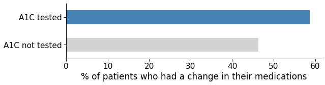
High HbA1c levels is one of the key indicators of diabetes. Maybe if the doctors asked for a test, they could see that a medication change was needed. The data shows that once A1c levels are assessed, a medication change is more likely to occur.
Conclusion
Both logistic regression and the random tree classifier were a good choice to address the problem of readmission of diabetic patients. This conclusion is given both by the good performance of both classifiers and by the insights that each one of them provided through the values of their coefficients.
Optimizing the hyperparameters was not a key step in gaining insights into the problem at hand, and the increase in the models’ score was negligible, especially in relation to logistic regression. As for the random tree classifier, the improvement in the ROC metric was relatively better, but with a huge impact on the model’s execution speed. If we just want to gain insight into the problem, perhaps a random forest with fewer trees will suffice. However, if we want a model capable of making predictions as accurately as possible, every infinitesimal improvement can count (as long as it doesn’t overly impact the execution time, obviously).
The features that proved to be most relevant for the prediction of the machine learning model were almost coincidentally those already used by the LACE methodology. Despite that, these were the key insights:
- Time in hospital (and indirectly the number of lab procedures, number of procedures, and number of medications) could indicate the patient’s health. The longer the stay, the higher the probability of being readmitted within 30 days.
- Number of inpatient visits in the last year could also be an indicator of the patient’s health, but longer term. It is also strongly correlated with early readmission.
- The older the patient, the higher the probability of early readmission after discharge.
- People who were discharged to their homes (instead of a skilled nursing facility, another short term hospital or clinic, etc.) are less likely to return within 30 days.
- Even after being diagnosed with diabetes-related symptoms, patients who did not have their HbA1c levels checked were more prone to early readmission, most likely because they needed a medication change.
Improvements
Future versions of this model could make use of NLP techniques to further improve its performance. More specifically, we could replace each diagnosis with a full medical description of each, including symptoms, and incorporate this new data into the original dataset.
For more information, please check out my Github repository containing the Jupyter notebook for technical details.
References
Cheng, S.-W., Wang, C.-Y., & Ko, Y. (2019). Costs and Length of Stay of Hospitalizations due to Diabetes-Related Complications. Journal of Diabetes Research, 2019, 1–6. https://doi.org/10.1155/2019/2363292
Graham, K. L., Auerbach, A. D., Schnipper, J. L., Flanders, S. A., Kim, S., Robinson, E. J., Ruhnke, G. W., Thomas, L. R., Kripalani, S., Vasilevskis, E. E., Fletcher, G. S., Sehgal, N. J., Lindenauer, P. K., Williams, M. V., Metlay, J. P., Davis, R. B., Yang, J., Marcantonio, E. R., & Herzig, S. J. (2018). Preventability of Early Versus Late Hospital Readmissions in a National Cohort of General Medicine Patients. Annals of Internal Medicine, 168(11), 766–774. https://doi.org/10.7326/M17-1724
Leppin, A. L., Gionfriddo, M. R., Kessler, M., Brito, J. P., Mair, F. S., Gallacher, K., Wang, Z., Erwin, P. J., Sylvester, T., Boehmer, K., Ting, H. H., Murad, M. H., Shippee, N. D., & Montori, V. M. (2014). Preventing 30-Day Hospital Readmissions: A Systematic Review and Meta-analysis of Randomized Trials. JAMA Internal Medicine, 174(7), 1095. https://doi.org/10.1001/jamainternmed.2014.1608
Robinson, R., & Hudali, T. (2017). The HOSPITAL score and LACE index as predictors of 30 day readmission in a retrospective study at a university-affiliated community hospital. PeerJ, 5, e3137. https://doi.org/10.7717/peerj.3137
Rubin, D. J. (2015). Hospital Readmission of Patients with Diabetes. Current Diabetes Reports, 15(4), 17. https://doi.org/10.1007/s11892-015-0584-7
Smeraglio, A., Heidenreich, P. A., Krishnan, G., Hopkins, J., Chen, J., & Shieh, L. (2019). “Patient vs provider perspectives of 30-day hospital readmissions.” BMJ open quality, 8(1), e000264. https://doi.org/10.1136/bmjoq-2017-000264
Soh, J. G. S., Wong, W. P., Mukhopadhyay, A., Quek, S. C., & Tai, B. C. (2020). Predictors of 30-day unplanned hospital readmission among adult patients with diabetes mellitus: A systematic review with meta-analysis. BMJ Open Diabetes Research & Care, 8(1), e001227. https://doi.org/10.1136/bmjdrc-2020-001227
Strack, B., DeShazo, J. P., Gennings, C., Olmo, J. L., Ventura, S., Cios, K. J., & Clore, J. N. (2014). Impact of HbA1c Measurement on Hospital Readmission Rates: Analysis of 70,000 Clinical Database Patient Records. BioMed Research International, 2014, 1–11. https://doi.org/10.1155/2014/781670
Swami, J., Donihi, A., Siminerio, L. M., French, E. K., Delisi, K., Hlasnik, D. S., Patel, N., Pinkhasova, D., Rubin, D. J., & Korytkowski, T. (2018). Readmission and Comprehension of Diabetes Education at Discharge (ReCoDED Study). Diabetes, 67(Supplement 1), 147-LB. https://doi.org/10.2337/db18-147-LB